For a quick idea of what you can do with this data, consider Kewley
et al's starburst criterion (2001ApJ...556..121K), which
compares [OIII]/Hb with ([SII]6716+[SII]6730)/Ha. In this example, we will
investigate where in the this plane our pixels lie.
We will use pyVO, TOPCAT, and Aladin.
Since we need to do somewhat complex operations on the image pixels,
we'll use pyVO to get the source images and convert them into a table of
fluxes. This table will then be investigated using TOPCAT (and a bit of
Aladin).
Produce a flux table: You could use Aladin for going from the images to a
table for fluxes, but this is a bit of drudgery here. Instead, here is a short
python script using pyVO and numpy; it uses TAP to retrieve the image metadata
and then get the images themselves by plain HTTP.
It then filters out all pixels with an SNR below 5 (with a bit of handwaving,
assuming what's ok in the generally weakest band will be ok in the others)
puts the remaining pixels into a nice relational table. It finally sends
this table to TOPCAT, so start TOPCAT before running this:
from astropy.io import fits as pyfits
from astropy import table, wcs
from pyvo import samp
import numpy
import pyvo


# change the following to use other ppakm31 fields
FIELD = "F3"


def stringify(s):
    """returns s utf-8-decoded if it's bytes, s otherwise.

    (that's working around old astropy votable breakage)
    """
    if isinstance(s, bytes):
        return s.decode("utf-8")
    return s


def get_image_metadata(field):
    """returns metadata rows from the ppakm31 service for field.

    Access URL and schema are taken from a TOPCAT exploration of the service.
    """
    svc = pyvo.dal.TAPService("http://dc.g-vo.org/tap")

    res = []
    for row in svc.run_sync(
            "select accref, field, imagetitle, bandpassid, cube_link"
            "  from ppakm31.maps"
            "  where field={}".format(repr(field))):
        res.append({
            "bandpassid": stringify(row["bandpassid"]),
            "accref": stringify(row["accref"]),})

    return res


def get_line_maps(image_meta):
    """returns a dict band->hdus for image_meta as returned by
    get_image_maps.
    """
    res = {}
    for row in image_meta:
        if row["bandpassid"]=='[NII]6583':
             # we don't need that one later, so skip it
             continue
        res[row["bandpassid"]] = pyfits.open(row["accref"])
    return res


if __name__=="__main__":
    line_maps = get_line_maps(get_image_metadata(FIELD))

    # Select pixels with a reasonable SNR; the errors are in extension
    # 1, and we use [OIII]5007, since the other lines ought to be stronger
    snr_cutoff = 5.
    snr_mask = (line_maps["[OIII]5007"][0].data
        > line_maps["[OIII]5007"][1].data*snr_cutoff)

    # The line maps all have identical WCS: use any to turn pixels to pos.
    # This is a somewhat tricky way to get the positions of all valid
    # pixels:
    w = wcs.WCS(header=line_maps["Halpha"][0].header, naxis=2)
    ras, decs = w.wcs_pix2world(
        snr_mask.nonzero()[1], snr_mask.nonzero()[0], 1)

    # Create table with ra & dec positions and our flux measurements.
    t = table.Table([
        ras,
        decs,
        line_maps["[OIII]5007"][0].data[snr_mask],
        line_maps["Hbeta"][0].data[snr_mask],
        line_maps["Halpha"][0].data[snr_mask],
        line_maps["[SII]6716"][0].data[snr_mask],
        line_maps["[SII]6730"][0].data[snr_mask]],
        names=('ra', 'dec', 'OIII_5007','Hbeta','Halpha','SII_6716','SII_6730'))

    # Send the table to TOPCAT via SAMP
    with samp.connection() as conn:
        samp.send_table_to(conn, t, "topcat")
You can change FIELD (or change the script so your flux table has all fields).
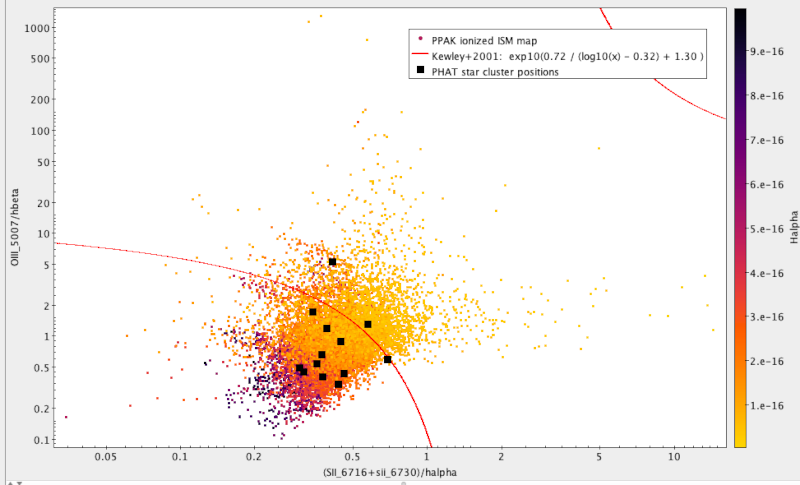
Make a plot of the line ratios: To visualise where the data likes
with respect to the Kewley+2001 criterion, once you have the table in TOPCAT,
configure the plot rougly likes this:
- Graphics → Plane Plot
- In X, type the denominator of the Kewley criterion; in case you forget how
the columns are called, check Views → Column Info. Anyway, it's
(SII_6716+SII_6730)/Halpha
- Similarly, for Y, use OIII_5007/Hbeta.
- In the Form tab, set the shading mode to aux, and set the Aux axis to
Halpha
- Under Axes, set both axes to log.
- Now add the Kewley criterion with Layers → Add Function Control and adding
using exp10(0.72/(log10(x)-0.32)+1.30) as the function to plot; to see
where this comes from, read 2001ApJ...556..121K.
The result would be something like this (see below for the black squares):
Sanity check: To see how the various points on your plot look in reality,
start Aladin and tell it to either some common survey or PPAKM31 images
themselves; you can find the latter in the discovery tree left in Aladin's
window.
Then, configure TOPCAT can make Aladin follow its focus by clicking Views →
Activation Action and then checking “Send Sky Coordinates”. See if you can
correlate the position in the plot with the visual (or infrared, or whatever)
appearance.
Compare to known clusters: To see what known star clusters fare in our plot,
get a catalogue of them. In TOPCAT, use VO → Cone Search, and in keywords,
enter something like “M31 cluster”; to find what we've plotted above,
J/ApJ/827/33, you'll have to check “description” in the match fields before
sending off the query (they don't mention M31 in their title or subject); but,
really, other catalogues of clusters or H II regions should do just as well.
To quickly get a position to search for, click into your plot; this will fill
out RA and Dec in the dialog, and all that's left is to enter, perhaps, 0.1 into
the radius field (because that's about the FoV of our images) and fire off the
request.
Whatever catalogue you used, the entries will probably not have the fluxes we
need to put them into our flux ratio plot. So: let's just add
them from our data by a positional crossmatch. To do that, in TOPCAT's main
window say Joins → Pair Match. Our pixel size is about 1 arcsec, so the default
match radius is ok. Select our fluxes as table 1 and the cluster catalogue as
table 2, hit “Go”, and then return to the flux plot.
In there, do Layers → Add position control. Configure this to plot the match
table, and again the flux expressions from above. If you then tell TOPCAT to
plot the points as large black squares, you will have reproduced (more or less)
the plot above.